Surface Geochemical Exploration (SGE) & Heat Flow Exploration


Leaders in SGE
Dr. Brooks et al. developed the analytical geochemistry of piston core samples at the Geochemical and Environmental Research Group (GERG) at Texas A&M University during the early 1980’s. Learn more about publications by TDI Brooks International staff.

SGE Coring

The piston-coring rig is comprised of a trigger assembly, the coring weight assembly, core barrels, tip assembly, and piston. The core barrels are in lengths of 6 and 9 meters. Expendable (used only once) butyrate tubes line the core-barrel and contain the sample.
|
# of Sections
|
Depth (cm)
|
Geochemical
Section(s) |
Archive Section
|
||
|
1
|
0-20
|
–
|
–
|
1
|
none
|
|
2
|
20-40
|
–
|
1
|
2
|
none
|
|
3
|
40-60
|
1
|
2
|
3
|
none
|
|
4
|
60-80
|
1
|
2
|
4
|
3
|
|
5
|
80-100
|
2
|
3
|
5
|
4
|
|
6
|
100-120
|
3
|
4
|
6
|
5
|
|
7
|
120-140
|
4
|
5
|
7
|
6
|
|
..
|
…….
|
..
|
..
|
..
|
..
|
|
30
|
580-600
|
15
|
21
|
30
|
29
|

Surface Heat Flow Measurements
Introduction to Heat Flow Exploration
Sample Heat Flow Distribution
Heat flow measurements serve critical purposes in oil exploration and production. The measured background or equilibrium heat flow, and measured sediment thermal conductivity provide strict constraints to geochemical models that determine regional scale maturation of basins with respect to oil and gas. In addition, area-wide heat flow surveys provide significant geological information on fluid flow from faults, lineaments, and around structures. Heat flow measurements in conjunction with seismic and sea floor geochemical studies provide a mechanism to assess fault and structural seals and contribute to a better understanding of regional hydrodynamics and hydrocarbon occurrence.
Heat Flow Probe
TDI-Brooks International has performed heat flow studies off the west African coast in Nigerian, Congolese and Angolan waters, in the Gulf of Mexico and in the Caribbean. TDI-Brooks International’s heat flow probe performs heat flow surveys in water depths up to 6000 m. In addition to measuring the sediment temperatures, the probe measures in situ thermal conductivity and water temperature profiles. The probe is capable of multiple measurements during a single 12-24 hour deployment. This one ton instrument is deployable from sea going vessels or platforms with a suitable winch and deployment system.
The heat flow in a region is due to heat moving upward from the mantle, together with thermal input from the radioactive decay of long-lived, naturally occurring isotopes in the earth’s crust. This conductive thermal regime is easily perturbed by the movement of fluids, which is the most effective form of heat transport. Thus, heat flow anomalies are indicative of recent or ongoing fluid flow in a sedimentary basin. Heat flow variations may also provide insight into basin stretching, sedimentation rates, and the presence of salt. Salt has a high thermal conductivity and thus enhances heat flow and perturbs maturation patterns and hydrodynamics around salt structures. In addition, the geotechnical stability of the ocean floor can be addressed as measured temperatures can determine the stability of gas hydrates in shallow sediments.
Description of Heat Flow Probe and Its Operation
Temperatures and temperature gradients within the sediment are measured by thermistors which are located at a known (30 cm) spacing within a small-diameter tube held in tension parallel to a solid steel strength member. Measurement of the thermal conductivity of the sediment is accomplished by (1) allowing the probe to remain at rest in the sediment to allow dissipation of the frictional heating generated by the penetration of the probe, and then (2) heating the probe and surrounding sediment by application of a fixed amount of energy to a heater wire that parallels the thermistors within the sensor tube. Analysis of the temperature decay following this period of energy input (or “heat pulse”) yields the conductivity of the sediment.
The Heat Probe consists of (1) instrumentation, consisting of 1-cm diameter sensor string tube, electronics data logger, heat pulse system, batteries, and pingers all contained within cylindrical pressure housings, (2) mechanical components, including weight stand and 6cm solid steel bar which extends continuously from wire termination at the top to the sensor tube support fin at the bottom, and (3) software with modules for communication, data analysis and graphic display. Further technical specifications are given in Appendix A.
Instrumentation
Instruments are contained in two interconnected pressure cases, one containing computer, measurement electronics, batteries and data logger and the other with pinger and battery. The probe contains sixteen (16) sensors (Fig. 1).
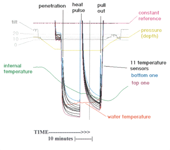
Figure 1. Annotated example of screen print of 16-sensor output.
Sensors 1-11. Temperatures, in milliKelvins (mK), measured within the probe at locations 30 cm apart, with sensor 1 the deepest, closest to the bottom of the sensor tube. These sensor temperatures appear as a cluster of 11 lines with the same value (water temperature during probe descent), until they divide into separate values when the probe enters the sediment. They respond very sharply to the heat pulse, and respond to frictional heating on probe penetration and pullout.
Sensor 12. Water temperature, in mK, measured by an external thermistor located at the top of the weight stand. On the displays, it generally tracks the 11 sensors in the sensor tube until the probe penetrates the sediment, then Sensor 12 remains constant at the bottom water temperature.
Sensor 13. The internal temperature of the probe electronics, in mK. This internal temperature is used to monitor internal conditions of the pressure case.
Sensor 14. The reference constant resistor, appearing at the very top of the display. It should remain constant, illustrating the stability of the electronic system. It is drawn on top of a straight line and is therefore only visible when the system is unstable.
Sensor 15. The tilt sensor, indicating the tilt of the probe from the vertical, in degrees, up to a maximum of 37.6°. A tilt greater than 37.6° is displayed as 37.6°. There are three horizontal lines near the top of the display, representing tilt values of 0°, 10°, and 20°. The tilt display changes from a maximum value (when the probe is horizontal on deck) to 0° when the probe is launched vertically into the water.
Sensor 16. The water pressure (depth) sensor, as measured by a quartz crystal sensor. At the surface, the water pressure appears at the middle tilt of the Sensor 15 reference line (10°). Note that for approximately three minutes before penetrating the sediment, the probe is held approximately 50 m above the bottom.
Electronics (Data Logger, Heat Pulse System, batteries, and pinger)
The controller is a 16-bit microprocessor and its operating program and normal default start-up configuration (number of channels, scan rate, etc.) is stored in ROM so that the system can be turned on and used immediately. Data from the sixteen sensors is passed through A/D converters and stored in RAM where there is sufficient memory to store 24 hours of continuous data. An on-board battery provides back up should there be a failure of the main battery system. The sealed lead-acid battery systems are recharged via an external connector at the end of each 24-hour operation period (without opening the pressure case). Old data are retained after data retrieval, and are overwritten only after an explicit command requiring verification. Data are retrieved via an external asynchronous 3-wire RS-232 connection at 9600 baud or via a simple delayed-ping acoustic telemetry scheme utilizing pinger with separate pressure case and power supply.
The heat pulse is software triggered only after the probe has penetrated the sediments and has remained stationary for a defined time interval (typically 7 minutes). This time interval allows the temperatures measured after penetration to approach equilibrium. Successful penetration and stationary period is represented by a constant pressure, as indicated by the pressure sensor. Pressure changes restart the time interval. However, once one heat pulse has been completed, further heat pulses are inhibited until the pressure sensor has indicated a pressure change of nominally ±10 meters. Heat pulses are also inhibited while the depth is less than 30 meters, to prevent heat pulses from occurring on deck. Power to the heater wire is applied for a programmable length of time (typically 20 seconds) beginning only after the probe has remained stationary for the desired time interval. The total power-time product delivered to the probe heater wire during a “heat pulse” is known, repeatable, and stable, with a target value of 600 joules/meter of probe length. Twenty properly regulated heat pulses per deployment are available.
Software: Communication and data analysis
Data are downloaded from the heat probe to the computer via the external asynchronous 3-wire RS-232 connection at 9,600 baud using the communication software PROCOMM, and data are graphically displayed using PRO40 (Figure 1). This program is also used pick penetration times and heat pulse parameters. Once data are arranged according to penetration time and heat pulse, data reduction is performed using a computer program (HFRED). This method was developed and described by Villinger and Davis (1987), following the method first suggested by Lister (1979). One shortcoming of this method is that the thermal conductivity is measured in the horizontal radial direction from the probe, whereas the value in the vertical direction is desired. As a result, anisotropy in the thermal conductivity of shale (including unconsolidated shale) and some other sediments can be considerable.
Mechanical Components
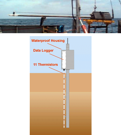
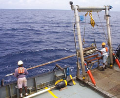
Figure 2. Heat flow probe
Figure 2 is a photograph of an assembled heat flow probe, resting in its cradle under the A-frame used to deploy it. The out-rigged thermistor string can been seen above and parallel to the solid steel strength member that penetrates the sediment. A diagram of the major components of the heat flow probe is also shown.
The length of probe is dictated by the “stiffness” of the sediments under investigation. A probe length of 3.5 meters is generally used for deep ocean work. This 6-cm diameter solid alloy steel bar extends continuously from the wire termination at the top through the weight stand and down to the sensor-tube support fin at the tip of the heat flow probe. The driving weight is provided by a 500 kg weight stand, constructed of galvanized steel and lead fill, which also houses and protects the instrument pressure cases. Access to all external connectors on the instrument cases is possible without removing the cylinders from the weight stand (i.e., for battery charging and RS-232 communications). The thermistor sensors and heater wire are contained within a high-strength 10-mm diameter stainless steel tube supported in tension 10 cm away from the strength member. The one ton instrument is usually suspended from a 9/16″ torque-balanced oceanographic wire. A universal swivel termination at the top of the heat flow probe prevents fouling of the wire around the weight stand with resulting damage to the sensor string. In addition to an adequate winch and A-frame deployment device, a tensiometer is used to determine definitively when the probe has penetrated the sediment (i.e. when the probe weight has come off the wire).
Operation
The heat flow system is modular in design and quickly assembled. The strength member is inserted through the weight stand and secured with a large nut and swivel/feegee assembly. The modular electronics packages are inserted in each end of the pressure housing. The assembled electronics package in its pressure housing is inserted in the weight stand and secured in place. The bulkhead connectors providing communications, battery recharge and input from water temperature and pressure sensors are accessible from the top of the weight stand. The probe may be charged, checked and test run on the ship before being placed in the water with real time feed back via the communications package.
At most stations the probe is lowered to within 50 m of the bottom, at a rate of 60 m/minute and held there for 3 minutes, then lowered into the bottom where it remains for 20 minutes, with the heat pulse occurring at the 10 minute stationary midpoint. In order to guarantee probe penetration at each site, the tensiometer is carefully monitored. Both during insertion when weight comes off the wire and during pullout, to ensure that pullout tension is much greater than the weight of the probe and cable.
Ambient temperatures below the seabed are derived by ten minute tracking of the heat decay induced by the frictional energy of the core barrel and mathematically projecting the resulting decline curve to infinity. The heat pulse is then applied to the cored section enabling the conductivity of each 30 cm section to be calculated using an identical ten minute sampling procedure. Heat flow (Q) measured in mW/m2 is determined by combining the site thermal conductivity (k) measured in W/m-K with the geothermal gradient (G) measured in mK/m determined from the thermistors according to the following relationship.
Water depth is measured by pressure and the angle of tilt of the core barrel is monitored to obtain true vertical depths.
Output
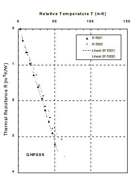
Figure 3. Comparison of heat flow measured by different electronics at a common station.
For each station, the data are immediately graphically displayed to evaluate effectiveness within minutes after probe data acquisition (Figure 1). Generally the resolution of the thermistors in the sensor tube is greatly amplified, so that fine details in the sediment temperatures can be viewed to ascertain that the data is of high quality.
A Bullard plot, a graph of sediment temperature (T) reported in mK versus the thermal resistance (R) reported in m2K/W, is output for each station. Thermal resistance is the integral of the inverse of thermal conductivity over the appropriate depth interval. Each plot illustrates the relative temperature as a function of the thermal resistance integrated from the top sensor downward through the sediment. The reciprocal of the slope of the resulting best-fit line is the heat flow (thermal resistance is plotted as the vertical Y parameter because it tracks depth; while heat flow is DT/DR), and under the ideal conditions of a constant vertical heat flow in a conductive regime, with isotropic thermal parameters, this would be a straight line.
The variance between sets of electronics is minimal as Bullard plots for a twice-sampled station indicates (Figure 3). The line slope from the Bullard plot is used to determine the most representative heat flow value for each station. At this station, the electronics were changed when the reference resistor measurements became unstable. The station was repeated with new electronics, and close heat flow results of 17.5 and 15.5 mW/m2 were obtained.
For the heat flow probe, the tilt sensor signal is recorded every 10 seconds, and during the time that the probe is in the sediment, it is generally constant. The magnitude of tilt, calibrated from 0 to 20° relative to vertical, is displayed on the sensor output print screen (Figure 1). To obtain the vertical heat flow, the tilt correction is the inverse of the cosine of the tilt angle. For stations with measured tilt less than 5° (which produces a correction factor of less than 1.004, or an increase in the heat flow of up to 0.4%), the correction is ignored. Tilt is almost always less than 5°.
Thermal Conductivity
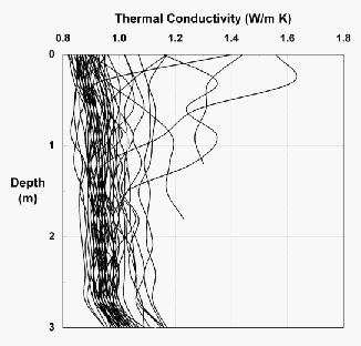
Figure 4. Thermal conductivity profiles in the sediments at each station.
At any point in the sediment column, the measured heat flow is the product of temperature gradient and thermal conductivity. The sediment thermal conductivity is mainly controlled by the water content of the sediment, since the thermal conductivity of water, 0.6 W/m-K, is much less than that of the rock matrix, which might typically be 2.3 W/m-K. For example, the thermal conductivities of Gulf of Mexico deep water stations, shown in Figure 4, typically range from 0.85 to 1.1 W/m-K, consistent with a variation in porosity from approximately 75 to 55% for the above assumed rock matrix thermal conductivity. The maximum thermal conductivity, of approximately 1.6 W/m-K, is consistent with a porosity of 25%. These measurements are accurate to 1% of value, so the measured variations are factual. The next most significant factor determining the thermal conductivity of the sediments is the amount of quartz in the sediments, since the thermal conductivity of quartz is very high.
Typical Results
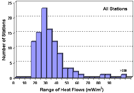
Figure 5. Distribution of measured heat flow values for Gulf of Mexico stations.
In the example of Figure 5, a set of Gulf of Mexico stations’ measured heat flows are plotted as a frequency bar chart. A generally well-behaved (Gaussian-like) distribution is typically observed in such a set, with a few outliers that are considered anomalies. In this sample set, the values are generally lower than the corrected heat flows of 41-47 mW/m2 obtained by Nagihara et al (1996). This is expected due to the higher sedimentation rates in this part of the Gulf of Mexico basin.
The Effect of Bottom Water Temperature
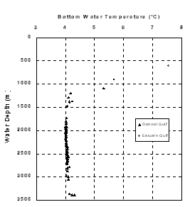
Figure 6. Water column temperatures as a function of depth.
As an example, a plot of the bottom water temperature (BWT) vs. water depth for various Gulf of Mexico stations (Figure 6) shows that the depth of minimum water temperature is between 1,900 and 2,300 m. This represents the maximum density of water, near 4oC. Below this depth, the water column in the Gulf of Mexico is more variable from place to place. At water depths of less than 1,500 m, larger temperature gradients appear. Eastern Gulf Stations at water depths of 902 and 604 m, respectively, have large variations in heat flow near the sediment-water interface, consistent with and controlled by past transients in the BWT.
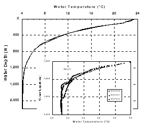
Figure 7. Small but significant differences in water temperatures measured down to a depth of 1,900 m at four Stations. Upper station has had a recent change in heat flux in the sediments, lower station illustrates three adjacent stations which had no changes in heat flux in sediments.
Eastern Gulf Stations at water depths of 1,373 and 1,412 m, respectively, have very constant heat flow in the upper 3 m of sediment, and show no sign of past transients in the BWT. However at one Station (1,472 m water depth), a small change in heat flow might be due to recent transients. Therefore, BWTs must be considered when evaluating the heat flow measurements in water depths less than approximately 1,000 m in this region of the Gulf of Mexico.
References
Keen, C.E. And T.J Lewis, Radiogenic heat production in sediments from the continental margin of eastern North America: Implications for hydrocarbon generation, American Association of Petroleum Geologists Bulletin, 66, 1402-1407, 1982.
Lewis, T.J., W.H. Bentkowski and J.A. Wright, Thermal State of Queen Charlotte Basin, British Columbia: Warm, in Evolution and Hydrocarbon Potential of the Queen Charlotte Basin, British Columbia, edited by G. Woodsworth, Paper 90-10, 489-506, Geological Survey of Canada, 1991.
Lister, C.R.B., The pulse-probe method of conductivity measurement, Geophysical Journal of the Royal Astronomical Society, 57, 451-461, 1979.
Nagihara, S., J.G. Sclater, J.D. Phillips, E.W. Behrens, T. Lewis, L.A. Lawver, Y. Nakamura, J. Garcia-Abdeslem and A.E. Maxwell, Heat flow in the western abyssal plain of the Gulf of Mexico: Implications for thermal evolution of the old oceanic lithosphere, Journal of Geophysical Research, 101, 2895-2913, 1996.
TDI-Brooks International, Inc., 1999 Central Gulf Consortium Heat -Flow Program, Basic Data Results, Tech. Rept. #99-303, 1999.
Villinger, H. and E.E. Davis, A new reduction algorithm for marine heat flow measurements, Journal of Geophysical Research, 92, 12,846-12,856, 1987a.
Villinger, H. and E.E. Davis, HFRED: A program for the reduction of marine hear flow data on a microcomputer, Geological Survey of Canada, Open File 1627, 78 pp, 1987b.
Appendix
HEAT FLOW PROBE SYSTEM SPECIFICATIONS
ELECTRONICS:
i) Power capacity and solid-state (no moving parts) logging of all data over a period of up to 24-hours.
ii) Tilt, pressure, and water-temperature measurements in addition to eleven sediment-temperature measurements.
iii) An acoustic data link capable of reliably transmitting data from depths to 5000 meters.
MECHANICAL DESIGN OF ELECTRONICS:
i) All electronics and batteries fit into a single, cylindrical pressure case. Nominal interior space is 6″ dia. x 26″ long.
ii) Modular construction of electronic functions should facilitate future upgrades and modifications, in particular to access the penetration (pressure) sensor, and possibly to expand the data logger and A/D functions.
OPERATIONAL REQUIREMENTS:
i) All normal daily operations, including communications, data retrieval, and battery charging can be accomplished without opening any of the pressure cases (i.e., via external underwater connectors).
ii) Electronics can function without adjustment over the temperature range; -5oC to +30oC.
iii) For test and normal operational purposes, some probe functions can be driven by software commands.
THERMISTORS:
i) Thermistors used for temperature measurement are YSI44032.
ii) Current through each thermistor during the measurement period is minimized to keep self-heating errors small.
iii) Thirteen temperature-equivalent channels are sampled. Eleven thermistors are in the probe itself, an additional separate thermistor for water temperature measurements is mounted on top of the instrument housing, and a fixed resistor is used as a reference “thermistor”.
iv) Each thermistor is individually connected to the electronics, reducing the chances of interference and mechanically induced failure of the sensor string.
THERMISTOR INTERFACE:
i) A minimum differential temperature resolution of +/- 1 moC, with +/-0.7 moC resolution typical, is available over a measuring temperature span of -5oC to +50oC.
ii) Values recorded are inversely proportional to the thermistor resistance. Resistance to temperature conversion is done external to the data logging operation, allowing individual resistance-to-temperature conversion parameters to be used for each thermistor if desired.
PRESSURE:
i) Pressure measurements over the depth range of 0 to 6000 meters are made, with better than 1 cm resolution of pressure change. Data storage of 24 bit words provide this resolution.
ii) A Paroscientific transducer Series 8B 7000-2 is used. The gauge is mounted in the instrument weight stand outside the pressure case.
iii) Only electrical wires from the pressure sensor penetrate the pressure case. Hydraulic tubing carrying external pressure is not brought into the interior of the pressure case.
TILT
i) Tilt measurements are made over the range 0o to 40o (from vertical) with a resolution of approximately 0.5o.
ii) The tilt transducer is located inside the pressure case.
TIME:
i) Real time (day/hour/min/sec) is recorded with the data. Time is accurate to within +/- 1 sec over 24 hours.
ii) Time is settable and checkable from outside the pressure case via an RS-232 data link.
iii) The real time clock is powered from an independent power source.
A/D CONVERSION AND SAMPLE RATE:
i) Sixteen-bit A/D converters are used in the electronics.
ii) Fastest scan rate (for 16 data channels – 11 thermistors, reference, water temperature thermistor, pressure, tilt, and time) is 1 scan/10 seconds. Scan rate is programmable (via an external RS-232 link) to include 1 scan per 10 to 60 seconds.
iii) All 16 data channels (11 probe thermistors, reference, water temperature thermistor, pressure, tilt, and time) are sampled within 1 second. In this manner, the time difference between sample times for each thermistor need not be taken into account.
CONTROLLER:
i) The controller is a 16-bit microprocessor chosen to allow flexibility and ease of modification.
ii) The operating program and normal default start-up configuration (number of channels, scan rate, etc.) is stored in ROM so that the system can be turned on and used immediately. Capability to change the configuration and issue operational commands is provided via a standard communications program. Access is gained through an RS-232 link at 9600 baud.
DATA STORAGE:
i) Data are stored in RAM. An on-board battery provides back-up should there be a failure of the main battery system. Old data are retained after data retrieval, and are overwritten only after an explicit command requiring verification.
ii) There is sufficient memory to store 24 hours of continuous data when scanning 16 channels (11 thermistors, reference resistor, water temp, pressure, tilt, and time) once every 10 seconds.
iii) Data storage ceases when memory is full.
DATA RETRIEVAL:
i) Data are retrieved via an external asynchronous 3-wire RS-232 connection at 9600 baud. Other speeds can be set.
HEAT PULSE CIRCUITRY:
i) Initiation of Heat Pulse: The heat pulse begins only after the probe has penetrated the sediments and has remained stationary for a time interval of approximately 7 minutes. This time interval is programmable (before deployment) in 1 minute increments between 5 and 15 minutes. This time interval allows the temperatures measured after penetration to approach equilibrium (to measure thermal gradient), and also allows pull-out of the probe before a heat pulse (application of the heat pulse for conductivity determination may not be required for all penetrations). Provision is also made for the test-firing of a heat pulse on deck with a user command.
ii) Detection of penetration and stationary period: A constant pressure, within +/- a programmable threshold (nominally 1 meter, programmable from 10 cm to 10 m), as indicated by the pressure sensor (see Section 6.0), is utilized to indicate a stationary penetration condition. Changes of more than the threshold restart the time interval period of Section 13.1. Once one heat pulse has been completed, further heat pulses are inhibited until the pressure sensor has indicated a pressure change of nominally +/-10 meters (i.e. after the probe has been withdrawn from the sediments; programmable from +/-1 to +/-10 meters). Heat pulses are also inhibited while the sensed depth is less than 30 meters (programmable), to prevent heat pulses from occurring while preparing the probe for deployment.
iii) Power to the heater wire: Current is applied for a programmable length of time (typically 20 seconds) beginning only after the probe has remained stationary for the desired interval (see Sec. 13.1). The length of the heat pulse is programmable in 1-second increments over the range 5 to 40 seconds.
iv) The time of application of the power to the heater wire is fixed in relation to the data scan cycle.
v) The total power-time product delivered to the probe heater wire during a “heat pulse” is known, repeatable, and stable, with a target value of 600 joules/(meter of probe length).
vi) Current is regulated at a level that is operator selectable in less than 1 A steps from about 1 to over 10 A. If the current falls below the regulated value, software and acoustic flags are set, alerting the operator to the condition.
vii) Total Number of Heat Pulses: The minimum number of available, properly regulated heat pulses per deployment is dependent on the state of charge of the batteries, and is typically 20.
ACOUSTIC TELEMETRY TRANSMISSION:
i) Type and Amount of Data Transmitted: As previously mentioned, reliability of a limited amount of data is more important than larger amounts of unreliable data. For this reason, a simple delayed-ping scheme has been implemented, with additional consideration given to future provision of a real-time ASCII-coded data for full-data transmission at a later date. The delayed-ping scheme works in the following manner: Only up to 5 channels of information (programmable, but typically tilt and temperature information from 3 thermistors) are transmitted. Each channel is allocated a 1-second information window. At the beginning of each second, a reference ping (5-ms pulse at 12 Khz) is transmitted, followed by a second ping where the time delay (0 to 1 sec) is proportional to the channel data value. For temperature, the conversion is nominally 10oC per second (i.e. there will be N-1 folds for a 10xN oC temperature span). This conversion is selectable from 1 to 10oC per second. For tilt the conversion is nominally 40o per second (i.e. no folding required for full-scale tilt).
ii) Telemetry Output: A simple contact closure of approximately 5 ms duration triggers a separate pinger having its own pressure case and power supply.
iii) Interference to Data Logging: Telemetry transmission does not interfere with, or induce errors in, the logged data. To ensure this, transmission and data acquisition do not occur simultaneously.
BATTERIES:
i) Sealed lead-acid batteries are utilized in the heat probe.
ii) Batteries can be charged via an external connector at the end of each 24-hour operation period without opening the pressure case.
iii) Battery chargers are supplied.
DOCUMENTATION:
i) Full documentation will be supplied for the operation and maintenance of the electronics, for operation of the system at sea.
ii) Programs to convert the raw data files downloaded from memory to a simple ASCII data file, and to view and subdivide data files are provided.
iii) Construction drawings are supplied for the mechanical assembly.
CALIBRATION AND INTEGRATION WITH MECHANICAL COMPONENTS:
i) The electronics are fully integrated into the pressure case, wired into pressure-case bulkhead connectors, and bench-tested with a thermistor string, external pressure sensor, and data-telemetry pinger.
ii) A calibration of the electronics using a high-precision decade resistance unit to simulate the characteristics of the thermistor string are completed and results provided. The result of this, and of the calibration of the tilt sensors are incorporated into the ASCII conversion program.
MECHANICAL CONSTRUCTION:
i) The structural member of the instrument is a 6 cm diameter solid alloy steel bar that extends continuously from the wire termination at the top to the sensor-tube support fin at the bottom.
ii) Driving weight is provided by a 500 kg monolithic weight stand, constructed of galvanized steel and lead fill, that also serves to house and protect the instrument pressure cylinders.
iii) Access to all external connectors on the instrument cylinders is possible without removing the cylinders from the weight stand (i.e., for battery charging and RS-232 communications).
iv) The thermistor sensors and heater wire are contained in a high-strength 10 mm diameter tube supported in tension 10 cm away from the strength member. Two spare sensor tube assemblies are supplied with the instrument.
v) The instrument must be tethered with a 13-mm (nominal diameter) coring wire. A universal swivel termination at the top of the heat probe is supplied. The Ship is required to supply a mating 13 mm yoke swivel wire termination.
Multibeam for Surface Geochemical Exploration (SGE)
Overview
Historically the design of SGE programs has relied on the use of regional 2D and 3D seismic data for the identification of potential surface seepage targets for core sample acquisition. While this technique has produced good results, seismic data has a number of drawbacks:
- High cost and operational complexity of acquisition;
- Limited areal coverage of the area of interest; and
- Low resolution
- Lower cost and operational complexity of acquisition
- 100% areal coverage of the area of interest;
- Very high resolution;
- Low probability of negative impact on marine mammals, environmental permitting issues reduced;
- Rapid turnaround time of data processing and interp / seep target selection;
- Can be used independently or in conjunction with 2D or 3D seismic data for seep target selection ; and
- Seeps can have a bathymetric or backscatter signature on the seafloor, or both.
TDI-Brooks and our partners have been involved in the design and execution of numerous ‘seep hunting’ MBES programs. TDI-Brooks operates two vessels with Kongsberg MBES systems, the RV Gyre and RV GeoExplorer, and has chartered third party vessels equipped with similar MBES systems suitable for seep hunting missions.
Intro to MBES Operations
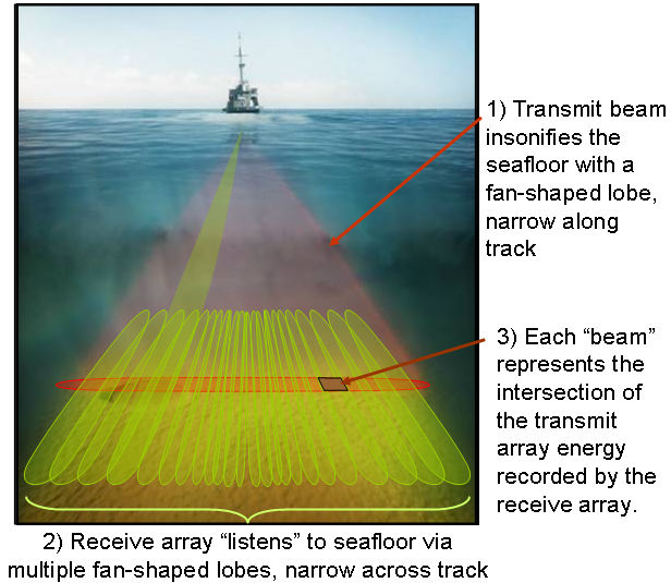
Multibeam echo sounders, like other sonar systems, emit sound waves in the shape of a fan from directly beneath a ship’s hull. These systems measure and record the time it takes for the acoustic signal to travel from the transmitter (transducer) to the seafloor (or object) and back to the receiver. In this way, multibeam sonars produce a “swath” of soundings (i.e., depths) for broad coverage of a survey area. Survey speed is typically higher than seismic operations (up to 10 kts).
 |
 |
| MBES operation and example of processed bathymetry data from EM710 on RV GeoExplorer | |
The area of coverage on the seafloor (swath) per ping depends on the depth of the water, seafloor composition, and the operating frequency of the multibeam sonar. Echosounders that transmit low frequency sound can travel a longer distance in the water (increased range and coverage) but have a lower resolution and are less precise. Sound from high-frequency echosounders cannot travel long distances in water but achieve a higher resolution and are more precise.
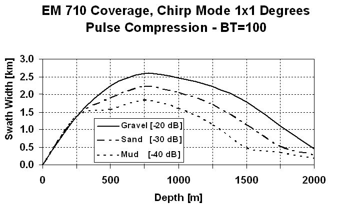
Expected range and coverage of a Kongsberg EM 710 MBES operating @ 70 – 100 kHz

Expected range and coverage of a Kongsberg EM 302 MBES operating @ 30 kHz
Most mid to deep water MBES systems are capable of meeting the resolution / data quality requirements for seep hunting missions. In general, lower frequency MBES systems will allow for increased coverage and reduce survey time, but this may be offset by higher vessel costs, as these system typically require a larger vessel to mount the transducer arrays than higher frequency systems (which use smaller transducer arrays).
The typical multibeam dataset for seep identification will consist of:
- Bathymetric surface grid (5 – 20m resolution)
- Quantitative backscatter grid (3 – 5m resolution)
- Water column plume data
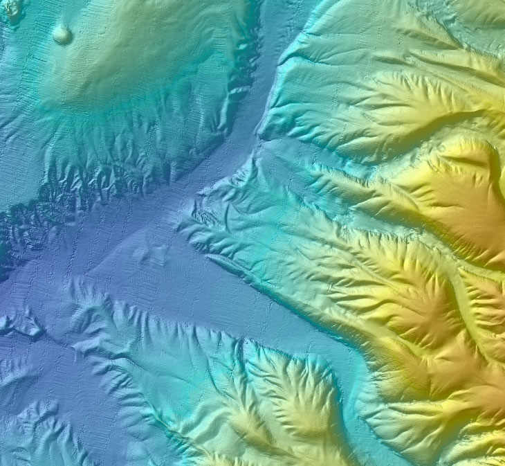
Bathymetric Surface Data
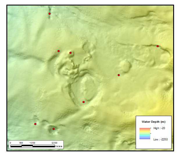
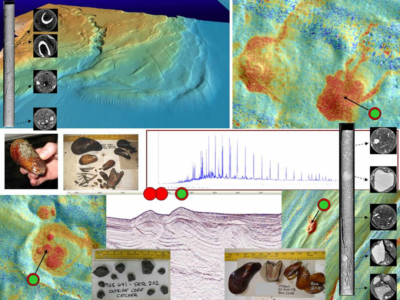
Bathymetry grid showing typical expulsion features (mounds and pockmarks).
Hydrocarbon seeps occur as point sources or clusters of point sources due to the vertical migration of hydrocarbons focusing into vertical chimneys. Hydrocarbons will follow a path of least resistance while migrating and therefore tend to form relatively small pathways compared to the overall volume of rock and sediments. As a result, surface expressions of seepage occur as discrete features, often with bathymetric character, such as a mud volcano or pockmark.
Backscatter Data
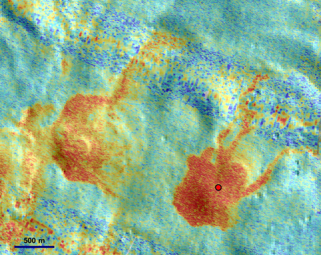
Multibeam backscatter grid draped over bathymetry surface, high backscatter values in red.
Backscatter is defined as the amount of acoustic energy being received by the sonar after interaction with the seafloor. This data can be used to characterize bottom type, because different bottom types “scatter” sound energy differently. For example, a softer bottom such as mud will return a weaker signal than a harder bottom, like rock.
While some surface seeps have an easily identifiable surface expression, there are many more occurrences with either very subdued or absent bathymetric response. Hydrocarbon seepage provides nutrients to chemosynthetic fauna, and also leads to precipitates such as authigenic carbonate, and, in appropriate temperature and pressure conditions, seafloor or near-seafloor gas hydrate. All of these conditions have an impact on the acoustic properties of the seafloor or the shallow sub-surface and can be identified by an elevated backscatter response. This backscatter response is the reason seep hunting works so well in the marine environment.
Water Column Data
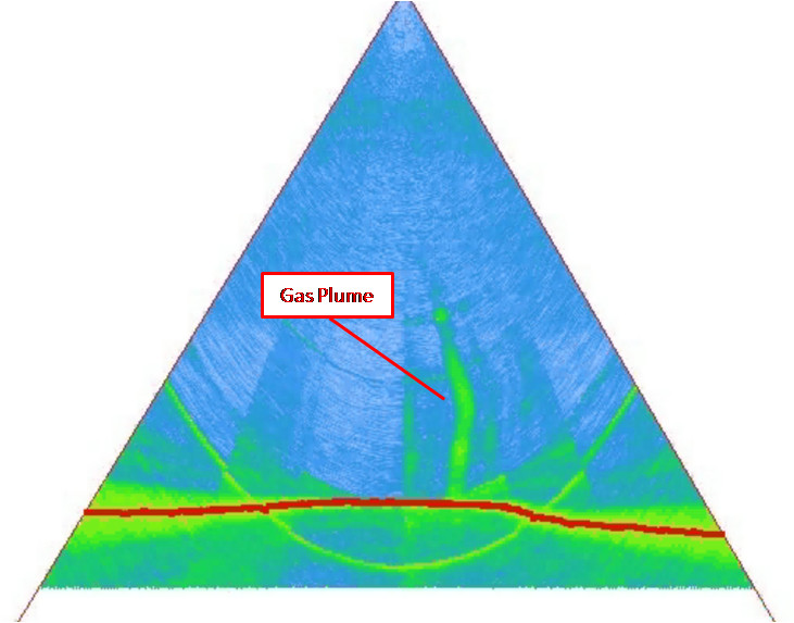
Gas plume detected in MBES water column data
In addition to recording the bottom return data (in the form of bathymetry and backscatter), many current generation MBES systems can record the returns throughout the entire water column. This data can be used to detect bubbles or gas plumes above the seafloor which could be indicative of hydrocarbon seepage. This plume data can be digitized and georeferenced to correlate with bathymetry and backscatter data.
When combined, MBES bathymetry, backscatter and water column data give trained interpreters a powerful and cost effective tool for identifying potential hydrocarbon seep sites.
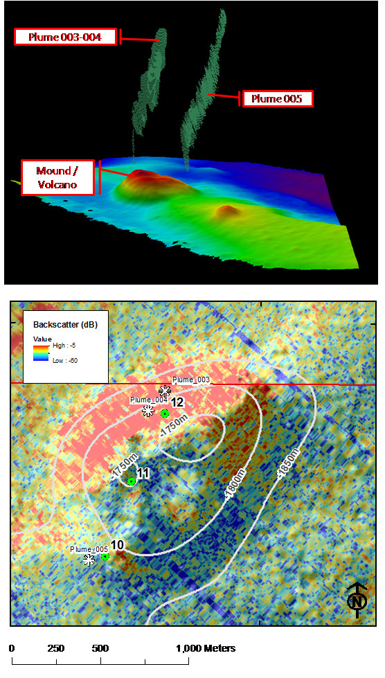
Integration of MBES bathymetry, backscatter and water column data for seep identification
SGE Publications

Dr. James M. Brooks
President & CEO
Abstract
Gas hydrates were recovered from eight sites on the Louisiana slope of the Gulf of Mexico. The gas hydrate discoveries ranged in water depths from 530 to 2400 m occurring as small to medium sized (0.5–50 mm) nodules, interspersed layers (1–10 mm thick) or as solid masses (> 150 mm thick). The hydrates have gas:fluid ratios as high as 170:1 at STP, C1/(C2 + C3) ratios ranging from 1.9 to > 1000 and δ13C ratios from −43 to −71‰. Thermogenic gas hydrates are associated with oil-stained cores containing up to 7% extractable oil exhibiting moderate to severe biodegradation. Biogenic gas hydrates are also associated with elevated bitumen levels (10–700 ppm). All gas hydrate associated cores contain high percentages (up to 65%) of authigenic, isotopically light carbonate. The hydrate-containing cores are associated with seismic “wipeout” zones indicative of gassy sediments. Collapsed structures, diapiric crests, or deep faults on the flanks of diapirs appear to be the sites of the shallow hydrates.


Dr. Bernie B. Bernard
Vice President & CTO
Abstract
Concentrations of the C1-C3 hydrocarbons and stable carbon isotope compositions of methane in recent sediments and seep gases of the Texas-Louisiana shelf-slope region were determined. These gases have been produced by both microbial and themocatalytic processes. Microbially-produced gases consist almost exclusively of methane, having C1/(C2+C3) hydrocarbon ratios greater than 1000 and δ13CPDB values of methane more negative than -60‰. Petroleum-related hydrocarbon gases generally have C1/(C2+C3) ratios smaller than 50 and isotopic ratios more positive than -50‰. A geochemical model based on these two parameters is used to show that natural gas compositions can be altered due to mixing of gases from the two sources as well as by microbial action and migration through sediments.
Light hydrocarbons in the upper few meters of Gulf of Mexico sediments are almost entirely of...
Bernard, B., 1978. Deep-Sea Research, Vol 26A, pp. 429 to 443.
Abstract
Interstitial methane profiles from six sediment cores taken on the slope and abyssal plain of the Gulf of Mexico can be explained by simple kinetic modeling. Methane is apparently produced at a constant rate and microbially consumed in the sulfate-reducing zone. Rates of production and consumption are estimated from best-fit solutions to a steady-state diagenetic equation. Production and consumption balance to form uniform concentrations of 5 to 10 µll-1 in the first few meters of slope and abyssal sediments. Effects of upward diffusion from large accumulations of methane in sulfate-free zones deeper than about 10m are not detectable.
Contact Us
TDI-Brooks International, Inc.
14391 S. Dowling Road
College Station, TX 77845
Email: info@tdi-bi.com
Phone: +1 (979) 693-3446
![]()
